Getting your data from one Hoja de cálculo de Google to another can be confusing. And while it can seem complex to do so, it is not difficult to learn effective ways to do so. Therefore, we created this article to help you learn how you can import all or part of your data from one Google Sheet to another.
We have gathered formulas from the simplest to advanced, including a way to pull all your data without getting lost in the rants of Google Sheet formulas.
We focused on three ways to help you, which will tackle how to pull your data from three different areas of your Google Sheets. These areas include:
- The data from one or more cells within your worksheet.
- Data from different tabs or worksheets.
- Data from other worksheets from different Google Sheets documents.
So, let’s check them out now.
Fast Forward:
- Simple functions for simple imports
- Advanced formulas to import your data in Google Sheets
- Using Dataslayer for Google Sheets
Simple functions for simple imports
These are the most basic formulas that are still helpful when you want to source some of your data from your worksheets. While they are so simple, they form the basis of other core functions in Google Sheets. So, skip to the other sections if you don’t need a refresher.
The best thing about them is you can replicate to other cells without doing the manual process of copying, pasting, and modifying your formulas into every cell that you want to reference from.
So, let’s now check out the formulas!
=CellReference
If you want to get data for a specific cell in a worksheet, you can use a direct cell reference formula to get its value. For example, if you want to get data from B3, you will use =B3 on the cell you need the data. Once you hit enter, your cell value will be imported.
Don’t know how you will replicate a formula into a range of cells? Follow this procedure:
- Place your cursor on the cell in your data destination worksheet that already contains your formula.
- Then drag it towards any direction you want to put your range.
- And that’s it! Your formula will now automatically adjust to the extended range.
=SheetName!CellReference
¡El conector de =sheetName!CellReference formula is a Google Sheets function that imports a cell value from a cell in other sheets (tabs) on the same document.
For example, if you want to fetch student names from another sheet within the same document, you will use =Students!B3. That means we want the value of cell B3 on the Students’ sheet.

Note: Put the name of the sheet in single quotes if it has spaces or other special characters, like !:;&*, etc.
={ReferenceRange}
If you need to import a specified range of data, you’ll use the ={ReferenceRange} formula. For example, ={A1:A4} will take data from A1 to A4 and maps it out to your sheet.
You can also use this formula to import data from another sheet in your workbook. For the above example, if the data was in the Students sheet, we will use ={Students!A1:A4}.
Note: Put the name of your sheet in single quotes if it has spaces or other special characters, like !:;&*, etc.
={SheetName!ColumnRange}
When you want to import a whole column to your workbook, you can use the column reference instead of the cell reference with the formulas above. Here’s how you can do it: ={Students!A:A}. This formula will import the whole column to your sheet.
You can use it to duplicate a column within a workbook by just using this formula with ={A:A}.
Advanced formulas to import your data in Google Sheets
There are two more formulas that are a bit advanced, but also easy to understand. So, let’s check them out.
Using the Filter function to Import data from one Google sheet to another based on criteria
Google Sheets FILTER function is one of the most frequently used functions in data operations. How it works is simple: it filters out subsets of data from a specified range using the criteria provided. But how can you use it to import data from other sheets? Let’s find out:
Note: The FILTER function and the Filter functionality in Google Sheets are not the same!
Syntax:
=FILTER(data_set,condition1, condition2,...)

Where:
data_range is the range of cells to filter.
condition is a criterion for the cell range that returns either TRUE or FALSE for the Filter function.
For example, to import data from another sheet using the FILTER function, you will do it this way:
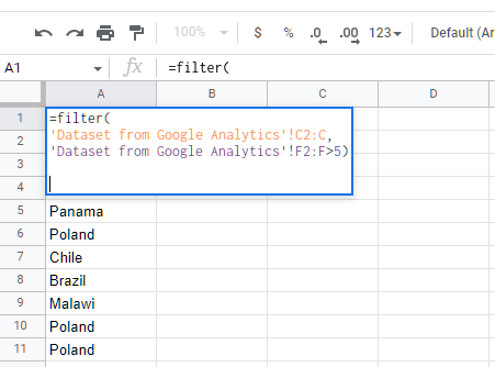
=filter(
'Dataset from Google Analytics'!C2:C,
'Dataset from Google Analytics'!F2:F>5)
This formula will return all the fields from a Google Sheet tab with the name ‘Dataset from Google Analytics.’ The data to be loaded is in column C, from C2 to the last cell, where F2:F is greater than five. This example is simple with a filter condition that uses simple comparison operators like >, =, and <.
While it is powerful, you can also nest conditions and make it as complex as required. You can also use the REGEXMATCH function to make it more functional.
If you need a detailed example of the FILTER function, check out this article.
Importing data from external spreadsheets with ImportRange in Google Sheet
The easiest way to import data from one google sheet to another is to use the IMPORTRANGE function. If you have data in separate sheets, the ImportRange formula can help you import your data within seconds.
So, to import your data from another Google sheet document, let’s follow along with an example.
Ready? Let’s get started.
The syntax for the ImportRange formula:
=IMPORTRANGE(“URL”, “SheetName!Range”)

Where:
URL is the link to the Google sheet spreadsheet for sourcing your data
SheetName is the name of your sheet if you have more than one in your workbook.
Range is the range of cells that you want to import into Google sheets.
For example:

To import cells D2 through to the last cell in that column from the first sheet of another Google Sheet document, we will use the formula this way:
=IMPORTRANGE("https://docs.google.com/spreadsheets/d/1Epmja02CeyXMiyBEuvGg8J_LAqjgaZWiGjEL3gqjCZw/edit#gid=1264662665","!D2:D")
Note: ImportRange formula has too many drawbacks with serious issues like reduced performance and usage limits that you should note when handling large datasets. Learn more about ImportRange’s best practices and its limitations here.
Using Dataslayer for Google Sheets
As we have checked the Google Sheets functions above, they are great and can help you solve most of your data imports and calculations. However, sometimes, these processes become repetitive or confusing that you would want a tool to make it a breeze.
Maybe you want to use advanced functionality that you could not achieve with Google Sheets formulas alone. Perhaps you also want to pull all your data to Google sheets from different sources for reporting — and google Sheets functions couldn’t be that efficient or effective for your needs.
So, you need a robust tool to help you where the functions could not surpass. Using a tool like Dataslayer para Google Sheets to import all your data in Google Sheets and across 40+ other data sources is perhaps the easiest and the most effective solution for you.
And the most effective way to import your Google sheets data into another sheet is to use Dataslayer for Google Sheets. If you have not yet set it up, here’s the process:

- On Google Sheets, tap on Extensions in the menu bar, hover on Add-ons, and click on Get Add-ons.
- Finally, hit the search icon and search for Dataslayer.
- On the search list, select Dataslayer and click Install.
Guide to getting started:
Once you have set it up, you will see Dataslayer is now added to your list of extensions. Click on it to launch it on the sidebar.
Then select Google Sheets as your data source.
After selecting Google Sheets, you’ll be prompted to enter the URL for the sheet you want to import your data from. So paste the link under the Report configuration field and click Get Data to Table.
And that’s it! You can customize your imported data with the options field. You can also schedule automatic refresh to maintain data freshness and email to get your updates whenever the data gets refreshed!
Conclusion
Importing your data from one Google sheet to another can be straightforward for simple references. However, complexity can turn in when you need to do it for multiple sheets with large rows of data.
We have discussed enough options for you to accomplish your data imports in Google Sheets for all your data, large or small.
If you are a regular Google Sheets user, a tool that will help you interconnect your sheets is indispensable for any data operation. No wonder, many Google sheets users will choose Dataslayer to make their data analysis faster and more efficient.
So, are you ready to try Dataslayer today? Join hundreds of others who have already found value from this powerful Google Sheets tool.