Ti sei mai chiesto quale formula puoi usare per unire tabelle in Google Sheets? E automaticamente? Il tipo di formula magica che sarebbe facile da riutilizzare e fa esattamente ciò di cui hai bisogno. Se vuoi sapere come — allora continua a leggere.
Every user finds it extremely important to find efficient Google Sheets formula that can work wonders for their data. However, it has been a challenge to get such effective formulas because chaining multiple functions can quickly create complex queries.
While many formulas are at our disposal, most require some creativity to make them ideal for your situations. So, when it comes to joining two or more tables, we have to depend on some other functions and reference knowledge to create a Google Sheets formula that can do the job effectively.
Se hai trovato il processo di unione delle tabelle noioso o complicato, questo articolo ti aiuterà a capire tutto ciò che devi sapere. Quindi, tuffiamoci subito in questa formula di Google Sheet per unire le tue tabelle!
What Google Sheets formula do you need to join tables?
Come abbiamo detto, unire due tabelle implica combinare diverse funzioni. La formula che costruiremo include due potenti funzioni di Google Sheets per unire le nostre tabelle: la FILTER e la VLOOKUP.
Come puoi vedere, le funzioni non sono nuove, ma quando le combini con alcuni altri trucchi, possono rivoluzionare il modo in cui elabori i tuoi dati più complessi. Prima di immergerci nella formula, dobbiamo consolidare la nostra comprensione di queste funzioni della query prima di poterla creare.
Quindi, rimbocchiamoci le maniche e mettiamoci al lavoro.
La funzione FILTER
Google Sheet formula FILTER is a powerful slice and dice function. The syntax for this function is:
=FILTER(intervallo, condizione1, [condizione2, …])
Dove:
- L'intervallo è l'intervallo di celle che desideri filtrare.
- Condizione1 è le righe o colonne che corrispondono al dataset e restituisce un array con valori booleani: i valori TRUE o FALSE in base alle tue condizioni.
- Condizione2: Sebbene questo sia un argomento facoltativo, svolge la stessa funzione di condizione1, aiutandoti a concatenare le condizioni.
La funzione FILTER restituisce la versione filtrata del tuo intervallo. Restituisce solo le righe o colonne che soddisfano le condizioni specificate che fornisci.
Quindi, se questa funzione può restituire una riga o una colonna in base alle nostre condizioni, sarà una delle nostre funzioni utili.
La funzione VLOOKUP
Quando vuoi fare riferimento a dati provenienti da fogli o tabelle diversi in Google Sheets, il VLOOKUP viene in aiuto. Questa funzione di ricerca verticale è potente e può lavorare con dati provenienti da fogli esterni, rendendola potente e perfetta per il nostro scopo.
You can use the Google Sheets formula VLOOKUP to source or lookup values that are matching on another table, so here’s the syntax:
=VLOOKUP(search_key, range, index, [is_sorted])
Dove:
- La chiave di ricerca: Il parametro search_key sono i valori che vogliamo cercare. Puoi inserire i dati, come 'Texas', 3400 o A12. Qui, puoi combinare valori provenienti da diverse colonne per ottenere una colonna di ricerca unica.
- L'intervallo: The second parameter in the VLOOKUP Google Sheets formula is the range: the references to cells where you want to search your data.
- L'indice: Un altro parametro nella funzione VLOOKUP è l'indice. L'indice è la posizione della colonna che desideri ottenere. Il numero della colonna inizia sempre dalla prima cella del tuo intervallo di ricerca, partendo da 1 e non da 0.
- Il parametro is_sorted: L'ultimo parametro in una funzione VLOOKUP è l'is_sorted. Questo parametro indica se dobbiamo ordinare la prima colonna in ordine crescente o meno. Quindi, i suoi valori possono essere FALSE o TRUE. Quando impostato su FALSE, l'intervallo di ricerca non sarà ordinato e rimarrà nell'ordine originale.
Illustrazione di VLOOKUP
To illustrate how to join a table using the Google Sheets formula VLOOKUP , we will use the following tables for our example. Here, we have two tables that share a common key, the Nome.
| A | B | |
| 1 | Nome | Dipartimento |
| 2 | Eric | Vendite |
| 3 | Jane | IT |
| 4 | John | Controllo Qualità |
| A | B | |
| 1 | Nome | Stipendio |
| 2 | Eric | $45500 |
| 3 | Jane | $31850 |
| 4 | John | $21440 |
If we need a Google Sheets formula to join the two tables above, here’s how we will achieve the results in Sheet C below:
| A | B | C | |
| 1 | Nome | Dipartimento | Stipendio |
| 2 | Eric | Vendite | $45500 |
| 3 | Jane | IT | $31850 |
| 4 | John | Controllo Qualità | $21440 |
Tabella A elenca i Nomi e Dipartimenti dei dipendenti. La seconda tabella elenca i Nomi e i loro Stipendio. Se hai bisogno di ottenere tutti questi dettagli in un'unica tabella, puoi usare VLOOKUP. Abbinerai ogni nome nella nuova Tabella C (Dove aveva il Nomi solo) con il nome corrispondente in FoglioB.
Come abbiamo fatto?
In B2 della Tabella C, we used this Google Sheets formula to get the Dipartimenti dei dipendenti:
=CERCA.VERT(A2,FoglioA!A2:B4,2,FALSO) e premi Invio.
Dove:]
A2 è la chiave di ricerca. FoglioA! è un riferimento a FoglioA con tabella A. A2:B4 è il nostro intervallo di ricerca su Foglio A. 2 è l'indice della colonna che vogliamo selezionare in A2:B4.
Su C2 di SheetC, use this Google Sheets formula to get the salary for the employees from FoglioB:
=CERCA.VERT(A2,SheetB!A2:B4,2,FALSO) e premi Invio.
Nota: Trascina la formula in altre celle per ottenere i loro valori.
Limitazioni della funzione VLOOKUP e come superarle
Diversi svantaggi derivano dall'uso della funzione VLOOKUP da sola. E se vuoi popolare l'intera colonna o riga senza farlo manualmente? E se i valori che stai cercando non sono unici? E se i valori che stai cercando non si trovano nella prima colonna del tuo intervallo?
There are two straightforward Google Sheets formula to deal with these limitations. Let’s check them out!
Utilizzando le concatenazioni
Le concatenazioni sono un modo per concatenare i valori di due o più celle in un unico valore. Quando le tue colonne hanno valori che non sono unici, questo può essere problematico per la funzione VLOOKUP. Pertanto, utilizzeremo le concatenazioni per creare colonne uniche affinché questa funzione funzioni in modo ottimale.
There are several ways to concatenate with Google Sheets formula, but we will only focus on the easiest: using the ampersand ‘&.’ For example, to concatenate cells A12 e A15, basta usare =A12&A15 come formula.
Because we want to do this virtually for our VLOOKUP Google Sheets formula, we will apply it to our search keys and range. So, let’s create another table with the following values:
| A | B | C | |
| 1 | Nome | Stato | Stipendio |
| 2 | Eric | Colorado | $40,500 |
| 3 | Jane | Connecticut | $37,600 |
| 4 | Eric | Delaware | $30,000 |
| 5 | John | California | $52,000 |
Se provi a duplicare o utilizzare VLOOKUP per popolare un'altra tabella senza valori unici, il valore della prima occorrenza della chiave di ricerca verrà utilizzato durante tutta la ricerca. Ecco l'esempio di utilizzo della tabella sopra per riprodurre la tabella. Controlla che il secondo Eric's Stato e Stipendio non sono accurati.
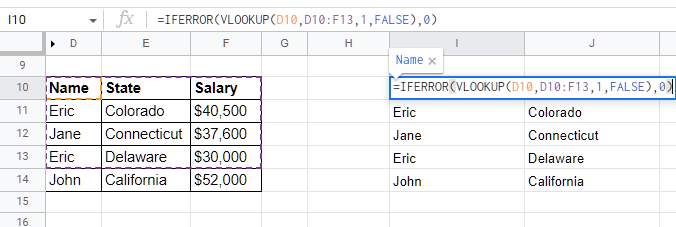
Per evitare tali errori, possiamo concatenare due celle o colonne per rendere la chiave unica, il che significa che avremo una maggiore possibilità di ottenere dati accurati. Abbiamo combinato il Nome e Stato per differenziare i due Eric in the list. Here’s the complete Google Sheets formula:
=VLOOKUP(H10&I10, {D10&E10, F10}, 2, FALSE)
Did you see we used the curly brackets to get that? What does it mean? To solve the other limitation of the Google Sheets formula VLOOKUP, we introduced the concept of arrays to allow us to create a virtual table and change the order of these tables without creating them manually.
Quindi, ecco la seconda soluzione alla limitazione:
Utilizzando gli array
Cosa sono gli array in Google Sheets? If you have a background in coding, you should know what an array means. However, it may mean different when you use it in Google Sheets formula. Arrays are tables with columns or rows of values.
Per differenziare una riga di valori da una colonna di valori in un array, si usa la virgola per rappresentare le colonne e il punto e virgola per rappresentare le righe. Se è confondente, ecco un esempio.
Se voglio rappresentare i nostri dati nell'ultima tabella in un array, una riga di Eric di Colorado sarà {Eric,Colorado,40500}. E le colonne di Nomi sono rappresentate come, {Eric;Jane;Eric;John}.
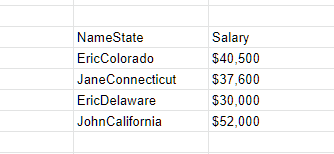
Tornando al nostro utilizzo sopra; dopo aver concatenato il Nomi e Stati, senza array sarà necessario creare un Colonna di Supporto to hold the concatenation. So, that is where arrays help us. With the arrays, we can now create a virtual column and use the VLOOKUP Google Sheets formula to use that table to get us the results we want.
Pertanto, la tabella virtuale dall'array {D10&E10, F10} significa che la tabella unirà i valori di D10 e E10 in una colonna e aggiungi il valore di F10 alla colonna successiva. Quindi, la tabella di aiuto completa dovrebbe apparire così:
Come gestire gli errori nei risultati
Even when everything might seem right, sometimes errors might behave awkwardly in Google Sheets formula. So, it is crucial to have a way to handle such issues. If you deal with a small dataset, you can find and fix the errors manually if it is well with you.
Un esempio di errore è il #N/A errore che si verifica quando la chiave di ricerca nella formula VLOOKUP non trova dati in una riga senza dati o quando la funzione FILTER non trova righe corrispondenti.
Fortunatamente, Google Sheets fornisce diverse formule per gestire tali errori. Ad esempio, l'IFNA troverà le celle con #N/A errors on your formula and replace them with a custom message. If you want to add zeros to such cells, here’s the Google Sheets formula:
Sintassi:
=IFNA(formula, “messaggio”)
Example, the Google Sheets formula:
=IFNA(FILTER(VLOOKUP(search_key,range,index,is_sorted), condition), “VLOOKUP non ha trovato alcun valore”)
Sebbene questo esempio possa sembrare ideale, annidare più formule di gestione degli errori può rendere le tue funzioni complicate. La buona notizia è che c'è un'alternativa: la funzione IFERROR, che è una sorta di universale per tutti gli errori.
The syntax and usage are just like IFNA; that is, the Google Sheets formula:
=IFERROR(formula, “messaggio”).
La nostra formula in azione: Unire due tabelle in Google Sheets
Ma ricordi la funzione FILTER che abbiamo introdotto prima? Dove si inserirà in questa formula?
Per rispondere a questo, lasciami presentarti un'altra limitazione della funzione VLOOKUP di cui non abbiamo discusso. La funzione VLOOKUP non popola automaticamente altre celle con valori— devi copiare e incollare o trascinare le formule per usarle in altre celle.
Ma questo è un altro lavoro che non vorrai fare. Quindi, come puoi superarlo? Ecco come puoi farlo:
=FILTRO(VLOOKUP(intervalloColonne,{array},indice o {array di indici},ordinato)Utilizzare la funzione FILTER per popolari i risultati di VLOOKUP
Utilizzando la funzione FILTER per filtrare i risultati di VLOOKUP con la condizione che l'intervallo non sia vuoto, sarai in grado di unire automaticamente le tue tabelle in Google Sheets.
Nel nostro esempio, la nostra funzione VLOOKUP trova i valori dall'intervallo che abbiamo fornito. La funzione FILTER eseguirà un ciclo su tutti i valori per ciascuna cella nell'intervallo di VLOOKUP fino a quando la condizione diventa falsa; cioè — quando VLOOKUP non restituisce nulla. La funzione FILTER popola quindi tutti i valori ricevuti nelle rispettive colonne nella nostra nuova tabella.
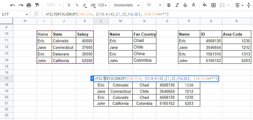
Come hai visto, abbiamo unito tre tabelle diverse utilizzando le funzioni VLOOKUP e FILTER. Ora, analizziamo le formule che abbiamo utilizzato:
La formula per ottenere Nome e Stato dalla Tabella 1:
=FILTRA(VLOOKUP(I10:I14, {I10:K14},{1,2},FALSO), I10:I14<>"")Qui, stiamo filtrando l'intervallo della colonna da I10:I14 dall'intervallo I10 a K14 con VLOOKUP. Poi includiamo un indice di array sulle colonne da cui vogliamo prelevare dall'intervallo; cioè indice colonna uno e due, {1,2}: Nome e Stato.
La formula per ottenere Paese Preferito da Tabella 2:
=FILTER(VLOOKUP(M10:M14, {M10:N14},2,FALSE), M10:M14"")Dal nostro intervallo M10:N10, vogliamo selezionare la seconda colonna (non da ordinare), e la nostra gamma di colonne M10:M14 non dovrebbe essere vuota secondo la nostra condizione FILTER.
Infine, la formula per ottenere ID e Codice Area da Tabella 3:
=FILTER(VLOOKUP(P10:P14, {P10:S14},{2,3},FALSE), P10:P14<>"")Riflessioni finali sulla query di Google Sheets per unire più tabelle
Merging two tables can be daunting, but with the functional Google Sheets formula that we shared to join your tables, we believe it’s now easier. By combining two powerful functions that we already know and use, the process is even more clear.
To merge different tables with Google Sheets formula, use the following syntax:
=FILTRA(VLOOKUP(intervallo_colonne, {intervallo_dati},{indice_colonne},ordinato), condizione) Se trovi ancora una difficoltà nell'utilizzare queste formule, considera di usare Dataslayer per Google Sheets, che ti consente di unire facilmente due tabelle, importare dati da diversi fogli di calcolo e lavorare con oltre 40 fonti di dati diverse per il tuo reporting. Vuoi saperne di più? Inizia oggi gratuitamente!