Obter seus dados de uma Google Sheet to another can be confusing. And while it can seem complex to do so, it is not difficult to learn effective ways to do so. Therefore, we created this article to help you learn how you can import all or part of your Google Sheets data from one sheet to another.
We have gathered formulas from the simplest to advanced, including a way to pull all your data without getting lost in the rants of Google Sheet data formulas.
We focused on three ways to help you, which will tackle how to pull your Google Sheets data from three different areas of your Sheets. These areas include:
- Os dados de uma ou mais células dentro da sua planilha.
- Dados de diferentes abas ou folhas de cálculo.
- Google Sheets data from other worksheets from different documents.
Então, vamos conferi-los agora.
Avançar Rápido:
- Funções simples para importações simples
- Fórmulas avançadas para importar seus dados no Google Sheets
- Usando o Dataslayer para Google Sheets
Funções simples para importações simples
These are the most basic formulas that are still helpful when you want to source some of your data from your worksheets. While they are so simple, they form the basis of other core functions in Google Sheets data. So, skip to the other sections if you don’t need a refresher.
A melhor coisa sobre elas é que você pode replicar para outras células sem fazer o processo manual de copiar, colar e modificar suas fórmulas em cada célula que você deseja referenciar.
Então, vamos agora conferir as fórmulas!
=ReferênciaDeCélula
Se você quiser obter dados de uma célula específica em uma planilha, pode usar uma fórmula de referência de célula direta para obter seu valor. Por exemplo, se você quiser obter dados de B3, você usará =B3 na célula onde você precisa dos dados. Assim que você pressionar enter, o valor da sua célula será importado.
Don’t know how you will replicate a formula into a range of cells in your Google Sheets data? Follow this procedure:
- Coloque o cursor na célula em sua planilha de destino de dados que já contém sua fórmula.
- Depois, arraste-o na direção que desejar para colocar seu intervalo.
- E é isso! Sua fórmula agora se ajustará automaticamente ao intervalo estendido.
=NomeDaFolha!ReferênciaDaCélula
O =nomedafolha!ReferênciaDaCélula a fórmula é uma função do Google Sheets que importa um valor de célula de uma célula em outras folhas (abas) no mesmo documento.
Por exemplo, se você quiser buscar nomes de alunos de outra folha dentro do mesmo documento, você usará =Alunos!B3. Isso significa que queremos o valor de célula B3 na a folha dos Alunos .
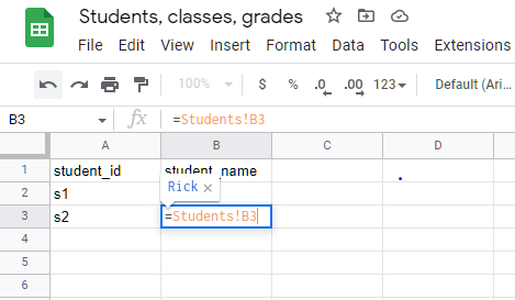
Nota: Coloque o nome da folha entre aspas simples se tiver espaços ou outros caracteres especiais, como !:;&*, etc.
={IntervaloReferência}
If you need to import a specified range of Google Sheets data, you’ll use the ={IntervaloReferência} fórmula. Por exemplo, ={A1:A4} irá pegar dados de A1 a A4 e mapeá-los na sua folha.
You can also use this formula to import data from another sheet in your workbook. For the above example, if the Google Sheets data was in the Students sheet, we will use ={Students!A1:A4}.
Nota: Coloque o nome da sua folha entre aspas simples se tiver espaços ou outros caracteres especiais, como !:;&*, etc.
={NomeDaFolha!IntervaloColuna}
Quando você quer importar uma coluna inteira para sua planilha, pode usar a referência da coluna em vez da referência da célula com as fórmulas acima. Aqui está como você pode fazer isso: ={Students!A:A}. Esta fórmula irá importar a coluna inteira para sua planilha.
Você pode usá-la para duplicar uma coluna dentro de um workbook usando apenas esta fórmula com ={A:A}.
Fórmulas avançadas para importar seus dados no Google Sheets
Há mais duas fórmulas que são um pouco avançadas, mas também fáceis de entender. Então, vamos dar uma olhada nelas.
Usando a função Filter para importar dados de uma planilha Google para outra com base em critérios
A função FILTER do Google Sheets é uma das funções mais frequentemente usadas em operações de dados. Como ela funciona é simples: ela filtra subconjuntos de dados de um intervalo especificado usando os critérios fornecidos. Mas como você pode usá-la para importar dados de outras planilhas? Vamos descobrir:
Nota: A função FILTER e a funcionalidade de Filter no Google Sheets não são iguais!
Sintaxe:
=FILTER(data_set, condição1, condição2,...)

Onde:
intervalo_de_dados é o intervalo de células a filtrar.
condição é um critério para o intervalo de células que retorna TRUE ou FALSE para a função Filter.
Por exemplo, para importar dados de outra folha usando a função FILTER, você fará assim:
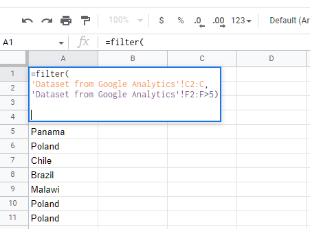
=filter(
'Dataset from Google Analytics'!C2:C,
'Dataset from Google Analytics'!F2:F>5)
This formula will return all the fields from a Google Sheets data tab with the name ‘Dataset from Google Analytics.’ The data to be loaded is in column C, de C2 até a última célula, onde F2:F é maior que cinco. This example is simple with a filter condition that uses simple comparison operators like >, =, and <.
Embora seja poderoso, você também pode aninhar condições e torná-las tão complexas quanto necessário. Você também pode usar o REGEXMATCH função para torná-la mais funcional.
Se você precisar de um exemplo detalhado do FILTER função, confira este artigo.
Importando dados de planilhas externas com ImportRange no Google Sheet
A maneira mais fácil de importar dados de uma planilha google para outra é usar o IMPORTRANGE função. Se você tiver dados em planilhas separadas, a fórmula ImportRange pode ajudar você a importar seus dados em segundos.
So, to import your data from another Google Sheets data document, let’s follow along with an example.
Pronto? Vamos começar.
A sintaxe da fórmula ImportRange:
=IMPORTRANGE("URL", "NomeDaFolha!Intervalo")

Onde:
URL é o link para a planilha do Google Sheets de onde você vai obter seus dados.
NomeDaAba é o nome da sua aba se você tiver mais de uma em sua pasta de trabalho.
Intervalo é o intervalo de células que você deseja importar para o Google Sheets.
Por exemplo:
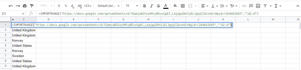
Para importar as células D2 até a última célula dessa coluna da primeira folha de outro documento do Google Sheets, usaremos a fórmula desta forma:
=IMPORTRANGE("https://docs.google.com/spreadsheets/d/1Epmja02CeyXMiyBEuvGg8J_LAqjgaZWiGjEL3gqjCZw/edit#gid=1264662665","!D2:D")Nota: A fórmula ImportRange tem muitos inconvenientes com sérios problemas como desempenho reduzido e limites de uso que você deve observar ao lidar com grandes conjuntos de dados. Saiba mais sobre as melhores práticas do ImportRange e suas limitações aqui.
Usando o Dataslayer para Google Sheets
Como verificamos as funções do Google Sheets acima, elas são ótimas e podem ajudá-lo a resolver a maioria de suas importações de dados e cálculos. No entanto, às vezes, esses processos se tornam repetitivos ou confusos, e você gostaria de uma ferramenta que tornasse isso fácil.
Talvez você queira usar funcionalidades avançadas que não conseguiu alcançar apenas com fórmulas do Google Sheets. Talvez você também queira importar todos os seus dados para o Google Sheets a partir de diferentes fontes para relatórios — e as funções do Google Sheets podem não ser tão eficientes ou eficazes para suas necessidades.
Portanto, você precisa de uma ferramenta robusta para ajudá-lo onde as funções não puderam superar. Usar uma ferramenta como Dataslayer para Google Sheets to import all your Google Sheets data and across 40+ other data sources is perhaps the easiest and the most effective solution for you.
E a maneira mais eficaz de importar seus dados do Google Sheets para outra folha é usar o Dataslayer para Google Sheets. Se você ainda não o configurou, aqui está o processo:
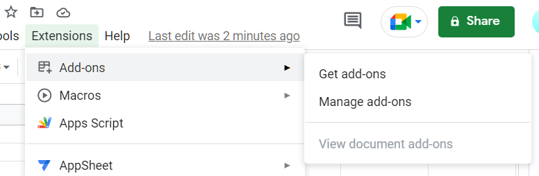
- No Google Sheets, toque em Complementos na barra de menu, passe o cursor sobre Complementos, e clique em Obter Complementos.
- Por fim, clique no ícone de pesquisa e procure por Dataslayer.
- Na lista de pesquisa, selecione Dataslayer e clique em Instalar.
Guia para começar:
Uma vez configurado, você verá que o Dataslayer agora foi adicionado à sua lista de extensões. Clique nele para lançá-lo na barra lateral.
Then select Google Sheets data as the source.
Após selecionar Google Sheets, você será solicitado a inserir a URL da planilha de onde deseja importar seus dados. Portanto, cole o link em a configuração do Relatório campo e clique em Obter Dados para Tabela.
E é isso! Você pode personalizar seus dados importados com o campo de opções. Você também pode agendar atualizações automáticas para manter a frescura dos dados e receber atualizações por e-mail sempre que os dados forem atualizados!
Conclusão
Importing your Google Sheets data to another sheet can be straightforward for simple references. However, complexity can turn in when you need to do it for multiple sheets with large rows of data.
We have discussed enough options for you to accomplish your Google Sheets data imports for all your data, large or small.
If you are a regular Google Sheets data user, a tool that will help you interconnect your sheets is indispensable for any data operation. No wonder, many Google sheets users will choose Dataslayer to make their data analysis faster and more efficient.
Então, está pronto para experimentar Dataslayer today? Join hundreds of others who have already found value from this powerful Google Sheets data tool.