


Já se perguntou qual fórmula você pode usar para unir tabelas no Google Sheets? E automaticamente? Aquele tipo de fórmula mágica que seria fácil de reutilizar e faz exatamente o que você precisa. Se você quer saber como — então continue lendo.
Every user finds it extremely important to find efficient Google Sheets formula that can work wonders for their data. However, it has been a challenge to get such effective formulas because chaining multiple functions can quickly create complex queries.
While many formulas are at our disposal, most require some creativity to make them ideal for your situations. So, when it comes to joining two or more tables, we have to depend on some other functions and reference knowledge to create a Google Sheets formula that can do the job effectively.
Se você achou o processo de juntar tabelas tedioso ou complicado, este artigo irá ajudá-lo a entender tudo o que você precisa saber. Então, vamos mergulhar diretamente nesta fórmula do Google Sheets para juntar suas tabelas!
What Google Sheets formula do you need to join tables?
Como dissemos, mesclar duas tabelas envolve combinar várias funções. A fórmula que iremos construir inclui duas funções poderosas do Google Sheets para unir nossas tabelas: o FILTER e o VLOOKUP.
Como você pode ver, as funções não são novas, mas quando combinadas com algumas outras dicas, podem revolucionar como você processa seus dados mais complexos. Antes de mergulharmos na fórmula, precisamos solidificar nossa compreensão dessas funções da consulta antes de podermos criá-la.
Então, vamos arregaçar as mangas e colocar mãos à obra.
A função FILTER
Google Sheet formula FILTER is a powerful slice and dice function. The syntax for this function is:
=FILTER(intervalo, condição1, [condição2, …])
Onde:
- O intervalo é o intervalo de células que você deseja filtrar.
- Condição1 são as linhas ou coluna que correspondem ao conjunto de dados e retornam um array com valores Booleanos: os valores TRUE ou FALSE com base nas suas condições.
- Condição2: Embora este seja um argumento opcional, ele serve a mesma função que condição1, ajudando você a encadear condições.
A função FILTER retorna a versão filtrada do seu intervalo. Ela retorna apenas as linhas ou colunas que atendem às condições especificadas que você fornece.
Portanto, se essa função pode retornar uma linha ou uma coluna com base em nossas condições, ela será uma de nossas funções úteis.
A função VLOOKUP
Quando você deseja se referir a dados de diferentes planilhas ou tabelas no Google Sheets, a função VLOOKUP é muito útil. Esta função de pesquisa vertical é poderosa e pode trabalhar com dados de planilhas externas, tornando-a poderosa e perfeita para o nosso propósito.
You can use the Google Sheets formula VLOOKUP to source or lookup values that are matching on another table, so here’s the syntax:
=VLOOKUP(search_key, range, index, [is_sorted])
Onde:
- A chave de busca: O parâmetro search_key são os valores que queremos buscar. Você pode inserir os dados, como 'Texas', 3400 ou A12. Aqui, você pode combinar valores de várias colunas para obter uma coluna de busca única.
- O intervalo: The second parameter in the VLOOKUP Google Sheets formula is the range: the references to cells where you want to search your data.
- O índice: Outro parâmetro na função VLOOKUP é o índice. O índice é a posição da coluna que você deseja obter. O número da coluna começa sempre a partir da primeira célula do seu intervalo de pesquisa, começando por 1 e não por 0.
- O parâmetro is_sorted: O parâmetro final em uma função VLOOKUP é o is_sorted. Este parâmetro indica se devemos classificar a primeira coluna em ordem crescente ou não. Portanto, seus valores podem ser FALSE ou TRUE. Quando definido como FALSE, o intervalo de pesquisa não será classificado e permanecerá na ordem original.
Ilustração do VLOOKUP
To illustrate how to join a table using the Google Sheets formula VLOOKUP , we will use the following tables for our example. Here, we have two tables that share a common key, the Nome.
| A | B | |
| 1 | Nome | Departamento |
| 2 | Eric | Vendas |
| 3 | Jane | TI |
| 4 | John | Controle de Qualidade |
| A | B | |
| 1 | Nome | Salário |
| 2 | Eric | $45500 |
| 3 | Jane | $31850 |
| 4 | John | $21440 |
If we need a Google Sheets formula to join the two tables above, here’s how we will achieve the results in Sheet C below:
| A | B | C | |
| 1 | Nome | Departamento | Salário |
| 2 | Eric | Vendas | $45500 |
| 3 | Jane | TI | $31850 |
| 4 | John | Controle de Qualidade | $21440 |
Tabela A lista os Nomes e Departamentos dos funcionários. A segunda tabela lista os Nomes e seus Salário. Se você precisar obter todos esses detalhes em uma tabela, pode usar o VLOOKUP. Você irá combinar cada nome na nova Tabela C (Onde tinha o Nomes único) com o nome correspondente na FolhaB.
Como conseguimos?
Em B2 da Tabela C, we used this Google Sheets formula to get the Departamentos dos funcionários:
=PROCV(A2,FolhaA!A2:B4,2,FALSO) e pressione Enter.
Onde:]
A2 é a chave de pesquisa. FolhaA! é uma referência a FolhaA com tabela A. A2:B4 é nosso intervalo de pesquisa em Folha A. 2 é o índice da coluna que queremos selecionar em A2:B4.
Ativar C2 de PlanilhaC, use this Google Sheets formula to get the salary for the employees from FolhaB:
=PROCV(A2,SheetB!A2:B4,2,FALSO) e pressione Enter.
Nota: Arraste a fórmula para outras células para obter seus valores.
Limitações da função VLOOKUP e como superá-las
Vários inconvenientes vêm com o uso da função VLOOKUP sozinha. E se você quiser preencher toda a coluna ou linha sem fazê-lo manualmente? E se os valores que você está procurando não forem exclusivos? E se os valores que você está procurando não estiverem na primeira coluna do seu intervalo?
There are two straightforward Google Sheets formula to deal with these limitations. Let’s check them out!
Usando concatenações
Concatenações são uma forma de encadear valores de duas ou mais células em um único valor. Quando suas colunas têm valores que não são únicos, isso pode ser problemático para a função VLOOKUP. Portanto, usaremos concatenações para criar colunas únicas para que essa função funcione de forma otimizada.
There are several ways to concatenate with Google Sheets formula, but we will only focus on the easiest: using the ampersand ‘&.’ For example, to concatenate cells A12 e A15, simplesmente use =A12&A15 como sua fórmula.
Because we want to do this virtually for our VLOOKUP Google Sheets formula, we will apply it to our search keys and range. So, let’s create another table with the following values:
| A | B | C | |
| 1 | Nome | Estado | Salário |
| 2 | Eric | Colorado | $40,500 |
| 3 | Jane | Connecticut | $37,600 |
| 4 | Eric | Delaware | $30,000 |
| 5 | John | Califórnia | $52,000 |
Se você tentar duplicar ou usar VLOOKUP para preencher outra tabela sem valores únicos, o valor da primeira ocorrência da chave de pesquisa será utilizado em toda a pesquisa. Aqui está o exemplo de uso da tabela acima para reproduzir a tabela. Verifique se o segundo Eric’s Estado e Salário não estão precisos.
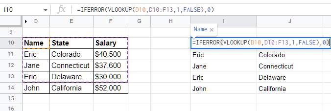
Para evitar tais erros, podemos concatenar duas células ou colunas para tornar a chave única, o que significa que teremos uma chance maior de obter dados precisos. Nós combinamos o Nome e Estado para diferenciar os dois Eric in the list. Here’s the complete Google Sheets formula:
=VLOOKUP(H10&I10, {D10&E10, F10}, 2, FALSO)
Did you see we used the curly brackets to get that? What does it mean? To solve the other limitation of the Google Sheets formula VLOOKUP, we introduced the concept of arrays to allow us to create a virtual table and change the order of these tables without creating them manually.
Então, aqui vem a segunda solução para a limitação:
Usando arrays
O que são arrays no Google Sheets? If you have a background in coding, you should know what an array means. However, it may mean different when you use it in Google Sheets formula. Arrays are tables with columns or rows of values.
Para diferenciar uma linha de valores de uma coluna de valores em um array, a vírgula é usada para representar colunas, e o ponto e vírgula representa as linhas. Se isso é confuso, aqui está um exemplo.
Se eu quiser representar nossos dados na nossa última tabela em um array, uma linha de Eric de Colorado será {Eric,Colorado,40500}. E as colunas de Nomes são representados como, {Eric;Jane;Eric;John}.
Voltando ao nosso uso acima; depois de concatenar o Nomes e Estados, sem arrays você precisará criar uma Coluna Auxiliar to hold the concatenation. So, that is where arrays help us. With the arrays, we can now create a virtual column and use the VLOOKUP Google Sheets formula to use that table to get us the results we want.
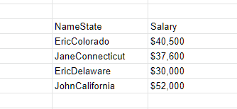
Portanto, a tabela virtual do array {D10&E10, F10} significa que a tabela irá mesclar os valores de D10 e E10 em uma coluna, e adicione o valor de F10 para a próxima coluna. Assim, a tabela auxiliar completa deve parecer com esta:
Como lidar com erros nos resultados
Even when everything might seem right, sometimes errors might behave awkwardly in Google Sheets formula. So, it is crucial to have a way to handle such issues. If you deal with a small dataset, you can find and fix the errors manually if it is well with you.
Um exemplo de erro é o #N/A erro que ocorre quando a chave de pesquisa na fórmula VLOOKUP não encontra dados em uma linha sem dados ou quando a função FILTER não encontra linhas correspondentes.
Felizmente, o Google Sheets fornece várias fórmulas para lidar com esses erros. Por exemplo, o IFNA encontrará as células com #N/A errors on your formula and replace them with a custom message. If you want to add zeros to such cells, here’s the Google Sheets formula:
Sintaxe:
=IFNA(fórmula, “mensagem”)
Example, the Google Sheets formula:
=IFNA(FILTER(VLOOKUP(chave_de_pesquisa, intervalo, índice, está_ordenado), condição), “VLOOKUP não encontrou valor”)
Embora este exemplo possa parecer ideal, aninhar várias fórmulas de tratamento de erros pode tornar suas funções complicadas. A boa notícia é que existe uma alternativa — a função IFERROR, que é uma espécie de universal para todos os erros.
The syntax and usage are just like IFNA; that is, the Google Sheets formula:
=IFERROR(fórmula, “mensagem”).
Nossa fórmula em ação: Unindo duas tabelas no Google Sheets
Mas você se lembra da função FILTER que apresentamos anteriormente? Onde ela se encaixará nesta fórmula?
Para responder a isso, deixe-me apresentar a você outra limitação da função VLOOKUP que não discutimos. A função VLOOKUP não preenche automaticamente outras células com valores — você precisa copiar e colar ou arrastar as fórmulas para usá-las em outras células.
Mas esse é outro trabalho que você não vai querer fazer. Então, como você pode superá-lo? Aqui está como você pode fazer isso:
=FILTRAR(PROCV(intervaloColuna;{array};índice ou {array de índices};está_ordenado))Usando a função FILTER para preencher os resultados do VLOOKUP
Usando a função FILTER para filtrar os resultados do VLOOKUP sob a condição de que o intervalo não esteja vazio, você poderá mesclar suas tabelas no Google Sheets automaticamente.
No nosso exemplo, a nossa função VLOOKUP encontra valores do intervalo que fornecemos. A função FILTER irá percorrer todos os valores para cada célula no intervalo VLOOKUP até que a condição se torne falsa; ou seja — quando o VLOOKUP não retornar nada. A função FILTER então preenche todos os valores recebidos nas suas respectivas colunas na nossa nova tabela.
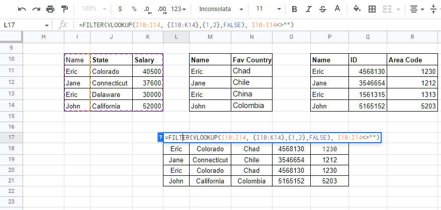
Como você viu, unimos três tabelas diferentes usando as funções VLOOKUP e FILTER. Agora, vamos analisar as fórmulas que utilizamos:
A fórmula para conseguir Nome e Estado da Tabela 1:
=FILTRAR(PROCV(I10:I14, {I10:K14},{1,2},FALSO), I10:I14"")Aqui, estamos a filtrar o intervalo de colunas de I10:I14 do intervalo I10 até K14 com VLOOKUP. Depois, incluímos um índice de array nas colunas que queremos escolher do intervalo; ou seja, índice de coluna um e dois, {1,2}: Nome e Estado.
A fórmula para conseguir País Favorito da Tabela 2:
=FILTER(VLOOKUP(M10:M14, {M10:N14},2,FALSE), M10:M14<>"")Da nossa gama M10:N10, queremos selecionar a segunda coluna (não a ser ordenada), e nosso intervalo de colunas M10:M14 não deve estar vazio de acordo com nossa condição FILTER.
Finalmente, a fórmula para obter ID e Código de Área da Tabela 3:
=FILTER(VLOOKUP(P10:P14, {P10:S14},{2,3},FALSE), P10:P14<>"")Considerações finais sobre a consulta do Google Sheets para unir mais tabelas
Merging two tables can be daunting, but with the functional Google Sheets formula that we shared to join your tables, we believe it’s now easier. By combining two powerful functions that we already know and use, the process is even more clear.
To merge different tables with Google Sheets formula, use the following syntax:
=FILTRAR(PROCV(intervalo_colunas, {intervalo_dados},{índice de colunas},ordenado), condição) Se você ainda encontra dificuldades em usar essas fórmulas, considere usar Dataslayer para Google Sheets, que pode permitir que você facilmente mescle duas tabelas, importe dados de diferentes planilhas e trabalhe com mais de 40 fontes de dados diferentes para o seu relatório. Quer saber mais? Comece hoje gratuitamente!


