Ever wondered which formula can you use to join tables in Google Sheets? And automatically? The kind of magic formula that would be easy to reuse and does exactly what you need. If you want to know how — then read on.
Every Google Sheets user finds it extremely important to find efficient formulas that can work wonders for their data. However, it has been a challenge to get such effective formulas because chaining multiple functions can quickly create complex queries.
While many formulas are at our disposal, most require some creativity to make them ideal for your situations. So, when it comes to joining two or more tables, we have to depend on some other functions and reference knowledge to create a query that can do the job effectively.
If you found the process of joining tables tedious or complicated, this article will help you understand everything you need to know. So, let’s dive right into this Google Sheet formula to join your tables!
What functions do you need to join tables in Google Sheets?
As we said, merging two tables involves combining several functions. The formula we will build includes two powerful Google Sheets functions to join our tables: the FILTER and the VLOOKUP.
As you can see, the functions are not new, but when combined them with a few other tricks, thus they can revolutionize how you process your most complex data. Before we dive into the formula, we need to solidify our understanding of these functions of the query before we can create it.
So, let’s roll our sleeves and get down to business.
The FILTER function
Google Sheet filter formula is a powerful slice and dice function. The syntax for this function is:
=FILTER(range, condition1, [condition2, …])
Where:
- The range is the range of cells that you want to filter.
- Condition1 is the rows or column that corresponds to the dataset and returns an array with Boolean values: the TRUE or FALSE values based on your conditions.
- Condition2: While this is an optional argument, it serves the same function as condition1, helping you chain conditions.
The FILTER function returns the filtered version of your range. It returns only the rows or columns that meet the specified conditions that you provide.
So, if this function can return a row or a column based on our conditions, it will be one of our useful functions.
The VLOOKUP function
When you want to refer to data from different sheets or tables in Google Sheets, the VLOOKUP function comes in handy. This vertical lookup function is powerful and can work with data from external sheets, making it powerful and perfect for our purpose.
You can use the VLOOKUP function to source or lookup values that are matching on another table, so here’s the syntax:
=VLOOKUP(search_key, range, index, [is_sorted])
Where:
- The search key: The search_key parameter is the values we want to look up for. You can enter the data, like ‘Texas’, 3400, or A12. Here, you can combine values from several columns to get a unique lookup column.
- The range: The second parameter in the VLOOKUP function is the range: the references to cells where you want to search your data.
- The index: Another parameter in the VLOOKUP function is the index. The index is the position of the column that you want to get. The column number always starts from the first cell of your search range, starting from 1 and not 0.
- The is_sorted parameter: The final parameter in a VLOOKUP function is the is_sorted. This parameter shows whether we should sort the first column in an ascending order or not. So, its values can either be FALSE or TRUE. When set to FALSE, the search range will not be sorted and remains in the original order.
VLOOKUP illustration
To illustrate how to join a table in Google Sheets using the VLOOKUP function, we will use the following tables for our example. Here, we have two tables that share a common key, the Name.
| A | B | |
| 1 | Name | Department |
| 2 | Eric | Sales |
| 3 | Jane | IT |
| 4 | John | Quality Control |
| A | B | |
| 1 | Name | Salary |
| 2 | Eric | $45500 |
| 3 | Jane | $31850 |
| 4 | John | $21440 |
If we need a Google Sheets query to join the two tables above, here’s how we will achieve the results in Sheet C below:
| A | B | C | |
| 1 | Name | Department | Salary |
| 2 | Eric | Sales | $45500 |
| 3 | Jane | IT | $31850 |
| 4 | John | Quality Control | $21440 |
Table A lists the Names and Departments of employees. The second table lists the Names and their Salary. If you need to get all these details in one table, you can use VLOOKUP. You will match each name in the new Table C (Where it had the Names only) with the corresponding name in SheetB.
How did we do it?
In B2 of Table C, we used this formula to get the Departments of the employees:
=VLOOKUP(A2,SheetA!A2:B4,2,FALSE) and hit Enter.
Where:]
A2 is the search key. SheetA! is a reference to SheetA with table A. A2:B4 is our search range on Sheet A. 2 is the index of the column we want to pick in A2:B4.
On C2 of SheetC, use this formula to get the salary for the employees from SheetB:
=VLOOKUP(A2,SheetB!A2:B4,2,FALSE)and hit Enter.
Note: Drag the formula to other cells to get their values.
Limitations of VLOOKUP function and how to overcome
Several drawbacks come with using the VLOOKUP function alone. What if you want to populate the whole column or row without doing it manually? What if the values you’re searching for are not unique? And what if the values you are looking for are not in the first column of your range?
There are two straightforward ways to deal with these limitations. Let’s check them out!
Using concatenations
Concatenations are a way of chaining up values of two or more cells into a single value. When your columns have values that are not unique, this can be problematic to the VLOOKUP function. Therefore, we will use concatenates to create unique columns for this function to work optimally.
There are several ways to concatenate in Google Sheets, but we will only focus on the easiest: using the ampersand ‘&.’ For example, to concatenate cells A12 and A15, simply use =A12&A15 as your formula.
Because we want to do this virtually for our VLOOKUP formula, we will apply it to our search keys and range. So, let’s create another table with the following values:
| A | B | C | |
| 1 | Name | State | Salary |
| 2 | Eric | Colorado | $40,500 |
| 3 | Jane | Connecticut | $37,600 |
| 4 | Eric | Delaware | $30,000 |
| 5 | John | California | $52,000 |
If you try to duplicate or use VLOOKUP to populate another table with no unique values, the value of the first occurrence of the search key will be used throughout the search. Here’s the example of using the table above to reproduce the table. Check that the second Eric’s State and Salary are not accurate.
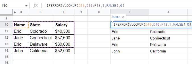
To avoid such errors, we can concatenate two cells or columns to make the key unique, meaning we will have a higher chance of getting accurate data. We combined the Name and State to differentiate the two Eric in the list. Here’s the complete formula:
=VLOOKUP(H10&I10, {D10&E10, F10}, 2, FALSE)

Did you see we used the curly brackets to get that? What does it mean? To solve the other limitation of the function VLOOKUP, we introduced the concept of arrays to allow us to create a virtual table and change the order of these tables without creating them manually.
So, here comes the second solution to the limitation:
Using arrays
What are arrays in Google Sheets? If you have a background in coding, you should know what an array means. However, it may mean different when you use it in Google Sheets. Arrays are tables with columns or rows of values.
To differentiate a row of values from a column of values in an array, the comma is used to represent columns, and the semicolon represents the rows. If it’s confusing, here’s an example.
If I want to represent our data in our last table in an array, a row of Eric of Colorado will be {Eric,Colorado,40500}. And the columns of Names are represented as, {Eric;Jane;Eric;John}.
Back to our usage above; after concatenating the Names and States, without arrays you will need to create a Helper Column to hold the concatenation. So, that is where arrays help us. With the arrays, we can now create a virtual column and use the VLOOKUP function to use that table to get us the results we want.
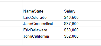
Therefore, the virtual table from the array {D10&E10, F10} means the table will merge the values of D10 and E10 in one column, and add the value of F10 to the next column. So, the complete helper table should look like this one:
How to handle errors in results
Even when everything might seem right, sometimes errors might behave awkwardly in Google Sheets. So, it is crucial to have a way to handle such issues. If you deal with a small dataset, you can find and fix the errors manually if it is well with you.
An example of an error is the #N/A error that happens either when the search key in the VLOOKUP formula found no data in a row with no data or when the FILTER function finds no matching rows.
Luckily, Google Sheets provides several formulas to deal with such errors. For example, the IFNA will find the cells with #N/A errors on your formula and replace them with a custom message. If you want to add zeros to such cells, here’s the formula:
Syntax:
=IFNA(formula, “message”)
Example:
=IFNA(FILTER(VLOOKUP(search_key,range,index,is_sorted), condition), “VLOOKUP found no value”)
While this example may seem ideal, nesting up multiple error-handling formulas can make your functions complicated. The good news is that there is an alternative — the IFERROR function, which is a sort of universal to all errors.
The syntax and usage are just like IFNA; that is,
=IFERROR(formula, “message”).
Our formula in action: Merging two tables in Google Sheets
But remember the FILTER function we introduced earlier? Where will it fit into this formula?
To answer that, let me introduce you to another limitation of the VLOOKUP function we haven’t discussed. VLOOKUP function does not automatically populate other cells with values— you need to copy and paste or drag the formulas to use them in other cells.
But that is another work you won’t want to do. So, how can you overcome it? Here is how you can do it:
=FILTER(VLOOKUP(columnRange,{array},index or {array of
indexes},is_sorted))
Using the FILTER function to populate the results of VLOOKUP
Using the FILTER function to screen the VLOOKUP results on the condition that the range is not empty, you will be able to merge your tables in Google Sheets automatically.
In our example, our VLOOKUP function finds values from the range that we provided. The filter function will loop all the values for each cell in the VLOOKUP range until the condition becomes false; that is — when VLOOKUP returns nothing. The FILTER function then populates all the values received to their respective columns in our new table.
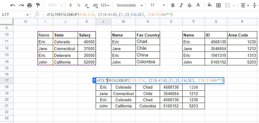
As you have seen, we have joined three different tables using VLOOKUP and FILTER functions. So, let’s now break down the formulas that we used:
The formula for getting Name and State from Table 1:
=FILTER(VLOOKUP(I10:I14, {I10:K14},{1,2},FALSE), I10:I14<>"")
Here, we are filtering the column range from I10:I14 from the range I10 to K14 with VLOOKUP. Then we include an array index on the columns we want to pick from the range; that is column index one and two, {1,2}: Name and State.
The formula for getting Fav Country from Table 2:
=FILTER(VLOOKUP(M10:M14, {M10:N14},2,FALSE), M10:M14<>"")
From our range M10:N10, we want to pick the second column (not to be sorted), and our column range M10:M14 should not be empty according to our FILTER condition.
Finally, the formula for getting ID and Area Code from Table 3:
=FILTER(VLOOKUP(P10:P14, {P10:S14},{2,3},FALSE), P10:P14<>"")
Final thoughts on the Google Sheets query to join more tables
Merging two tables can be daunting, but with the functional Google Sheets query that we shared to join your tables, we believe it’s now easier. By combining two powerful functions that we already know and use, the process is even more clear.
To merge different tables in Google sheets, use the following syntax:
=FILTER(VLOOKUP(columnrange, {datarange},{index of
columns},is_sorted), condition)
If you still find a challenge using these formulas, consider using Dataslayer for Google Sheets, which can allow you to easily merge two tables, import data from different spreadsheets, and work with over 40 different data sources for your reporting. Do you want to learn more? Get started today for free!